堆叠双重差分模型方法
1 堆叠DID(stacked DID)和多期DID(staggered DID)的区别 1.1 Difference in data
Sample windows: 2001 - 2005
Adoption year
stkcd
Group type
1999
1
Always treated
2002
2
Early treated
2004
3
Late treated
.
4
Never treated
Staggered DID panel data (N = 4 $\times$ 5 = 20)
stkcd
year
y
DID
Treat
Adoption year
1
2001
55
1
1
1999
1
2002
64
1
1
1999
1
2003
21
1
1
1999
1
2004
45
1
1
1999
1
2005
67
1
1
1999
2
2001
82
0
1
2002
2
2002
63
1
1
2002
2
2003
78
1
1
2002
2
2004
99
1
1
2002
2
2005
51
1
1
2002
3
2001
54
0
1
2004
3
2002
36
0
1
2004
3
2003
41
0
1
2004
3
2004
65
1
1
2004
3
2005
94
1
1
2004
4
2001
76
0
0
.
4
2002
37
0
0
.
4
2003
11
0
0
.
4
2004
76
0
0
.
4
2005
44
0
0
.
Stacked DID panel data (N = 3 $\times$ 10 = 30)
stkcd
year
y
DID
Treat
Adoption year in cohort
Cohort
1
2001
55
1
1
1999
1
1
2002
64
1
1
1999
1
1
2003
21
1
1
1999
1
1
2004
45
1
1
1999
1
1
2005
67
1
1
1999
1
4
2001
76
0
0
.
1
4
2002
37
0
0
.
1
4
2003
11
0
0
.
1
4
2004
76
0
0
.
1
4
2005
44
0
0
.
1
2
2001
82
0
1
2002
2
2
2002
63
1
1
2002
2
2
2003
78
1
1
2002
2
2
2004
99
1
1
2002
2
2
2005
51
1
1
2002
2
4
2001
76
0
0
.
2
4
2002
37
0
0
.
2
4
2003
11
0
0
.
2
4
2004
76
0
0
.
2
4
2005
44
0
0
.
2
3
2001
54
0
1
2004
3
3
2002
36
0
1
2004
3
3
2003
41
0
1
2004
3
3
2004
65
1
1
2004
3
3
2005
94
1
1
2004
3
4
2001
76
0
0
.
3
4
2002
37
0
0
.
3
4
2003
11
0
0
.
3
4
2004
76
0
0
.
3
4
2005
44
0
0
.
3
1.2 Difference in specification
Staggered DID specification
$$
where
$y_{it}$ is the outcome variable
$DID_{it}$ is the event dummy variable
$Controls_{it}$ is a vector contains a series of variables
$\delta_i$ and $\lambda_t$ are firm and year fixed effect, respectively
Reduced form
$$
where
$c$ is the cohort of firm $i$
$\delta_{ic}$ and $\lambda_{tc}$ are firm-cohort and year-cohort interacted fixed effect, respectively
Event study form
$$
where
$A_c$ is the adoption year of cohort $c$
$I()$ is an indicator function, equaling 1 when the inner equation holds
or more specifically
2 偏误的来源
Two assumption for common trend
Time-varying confounders must affect outcomes in both groups in the same way. -> Time fixed effects
Group-varying confounders must be time-invariant. -> Group fixed effects
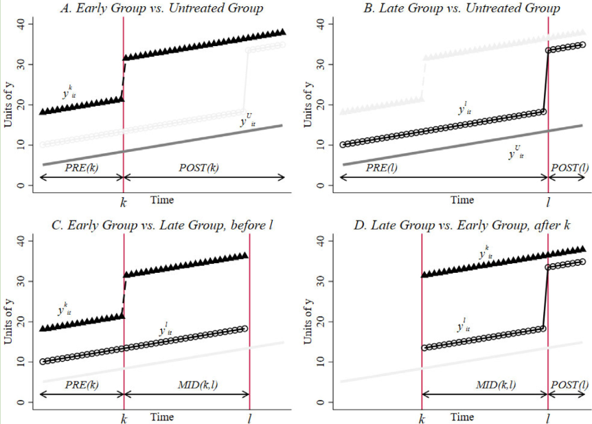
Goodman-Bacon, A. (2021). Difference-in-differences with variation in treatment timing. Journal of Econometrics, 225(2): 254-277.
Because the early group (bad control) is treated as a control group
See more details in Staggered Adoption Designs and Stacked DID and Event Studies (Coady Wing, 2021)
3 Stata code 3.1 Staggered DID
1
2
3
4
5
cd "D:\code\Stata\stackeddid" use "demo.dta" , clear reghdfe y did, a(stkcd year) vce (cl stkcd)
1
2
3
4
5
6
7
8
9
10
11
12
13
14
15
16
17
18
19
20
21
22
23
24
25
26
27
28
29
. reghdfe y did, a(stkcd year) vce (cl stkcd) (MWFE estimator converged in 2 iterations) HDFE Linear regression Number of obs = 20 Absorbing 2 HDFE groups F ( 1, 3) = 17.15 Statistics robust to heteroskedasticity Prob > F = 0.0256 R-squared = 0.5608 Adj R-squared = 0.1656 Within R-sq. = 0.0988 Number of clusters (stkcd) = 4 Root MSE = 20.9805 (Std. err . adjusted for 4 clusters in stkcd) ------------------------------------------------------------------------------ | Robust y | Coefficient std. err . t P>|t| [95% conf . interval] -------------+---------------------------------------------------------------- did | 19.26923 4.65359 4.14 0.026 4.459429 34.07903 _cons | 47.35192 2.559475 18.50 0.000 39.20653 55.49731 ------------------------------------------------------------------------------ Absorbed degrees of freedom: -----------------------------------------------------+ Absorbed FE | Categories - Redundant = Num. Coefs | -------------+---------------------------------------| stkcd | 4 4 0 *| year | 5 0 5 | -----------------------------------------------------+
3.2 Stacked DID
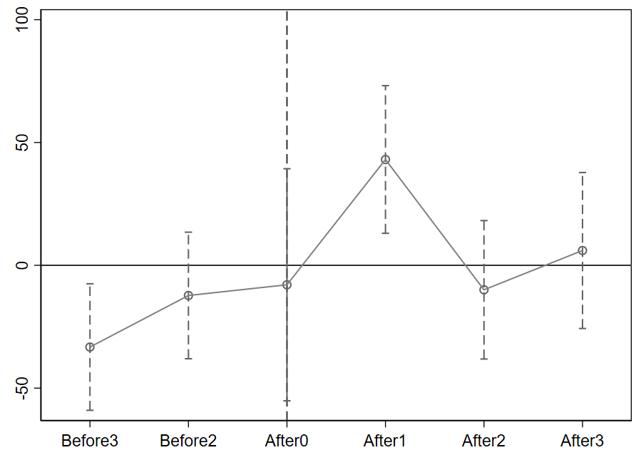
1
2
3
4
5
6
7
8
9
10
11
12
13
14
15
16
17
18
19
20
21
22
23
24
25
26
27
28
29
30
31
32
33
34
35
36
37
38
39
40
41
42
43
44
45
46
47
48
49
50
51
52
53
54
55
56
57
58
59
60
61
62
63
64
65
66
67
cd "D:\code\Stata\stackeddid" use "demo.dta" , clear drop if adoptionyear == 2002drop if adoptionyear == 2004gen cohort = 1save "cohort1.dta" , replace use "demo.dta" , clear drop if adoptionyear == 1999drop if adoptionyear == 2004gen cohort = 2save "cohort2.dta" , replace use "demo.dta" , clear drop if adoptionyear == 1999drop if adoptionyear == 2002gen cohort = 3save "cohort3.dta" , replace append using "cohort1.dta" append using "cohort2.dta" sort cohort stkcd yearsave "stackedmain.dta" , replace reghdfe y did, a(stkcd#cohort year#cohort) vce (cl stkcd) forvalue i = 3(-1)2{ gen Before`i' _ = cond (year - adoptionyear <= -`i' & adoptionyear != ., 1, 0) } forvalue i = 3(-1)1{ gen Before`i' = cond (year - adoptionyear == -`i' , 1, 0) } forvalue i = 0(1)3{ gen After`i' = cond (year - adoptionyear == `i' , 1, 0) } forvalue i = 2(1)3{ gen After`i' _ = cond (year - adoptionyear >= `i' & adoptionyear != ., 1, 0) } reghdfe y Before3 Before2 After0 After1 After2 After3, a(stkcd#cohort year#cohort) vce (cl stkcd) est store m1coefplot m1, keep (Before3 Before2 After0 After1 After2 After3) levels (90) vertical yline(0) xline(3, lp(dash)) addplot(line @b @at) ciopts(lpattern(dash) recast (rcap) msize(medium)) msymbol(circle_hollow) scheme(s1mono)
1
2
3
4
5
6
7
8
9
10
11
12
13
14
15
16
17
18
19
20
21
22
23
24
25
26
27
28
29
30
31
32
33
34
35
36
37
38
39
40
41
42
43
44
45
46
47
48
49
50
51
52
53
54
55
56
57
58
59
60
61
62
63
64
. reghdfe y did, a(stkcd#cohort year#cohort) vce (cl stkcd) (MWFE estimator converged in 2 iterations) HDFE Linear regression Number of obs = 30 Absorbing 2 HDFE groups F ( 1, 3) = 89.20 Statistics robust to heteroskedasticity Prob > F = 0.0025 R-squared = 0.7619 Adj R-squared = 0.1367 Within R-sq. = 0.0929 Number of clusters (stkcd) = 4 Root MSE = 22.3113 (Std. err . adjusted for 4 clusters in stkcd) ------------------------------------------------------------------------------ | Robust y | Coefficient std. err . t P>|t| [95% conf . interval] -------------+---------------------------------------------------------------- did | 20.2 2.138754 9.44 0.003 13.39353 27.00647 _cons | 47.49333 .7842096 60.56 0.000 44.99763 49.98904 ------------------------------------------------------------------------------ Absorbed degrees of freedom: --------------------------------------------------------+ Absorbed FE | Categories - Redundant = Num. Coefs | ----------------+---------------------------------------| stkcd#cohort | 6 6 0 *| year#cohort | 15 0 15 | --------------------------------------------------------+ . reghdfe y Before3 Before2 After0 After1 After2 After3, a(stkcd#cohort year#cohort) vce (cl stkcd) (MWFE estimator converged in 2 iterations) warning: missing F statistic; dropped variables due to collinearity or too few clusters HDFE Linear regression Number of obs = 30 Absorbing 2 HDFE groups F ( 6, 3) = . Statistics robust to heteroskedasticity Prob > F = . R-squared = 0.8914 Adj R-squared = -0.0501 Within R-sq. = 0.5863 Number of clusters (stkcd) = 4 Root MSE = 24.6071 (Std. err . adjusted for 4 clusters in stkcd) ------------------------------------------------------------------------------ | Robust y | Coefficient std. err . t P>|t| [95% conf . interval] -------------+---------------------------------------------------------------- Before3 | -33.27778 10.94557 -3.04 0.056 -68.11146 1.555902 Before2 | -12.27778 10.94557 -1.12 0.344 -47.11146 22.5559 After0 | -7.916667 20.0721 -0.39 0.720 -71.79504 55.96171 After1 | 43.08333 12.77056 3.37 0.043 2.441714 83.72495 After2 | -9.972222 11.97396 -0.83 0.466 -48.0787 28.13425 After3 | 6.027778 13.48936 0.45 0.685 -36.90138 48.95693 _cons | 54.33704 3.490034 15.57 0.001 43.23019 65.44388 ------------------------------------------------------------------------------ Absorbed degrees of freedom: --------------------------------------------------------+ Absorbed FE | Categories - Redundant = Num. Coefs | ----------------+---------------------------------------| stkcd#cohort | 6 6 0 *| year#cohort | 15 0 15 | --------------------------------------------------------+
4 参考文献
Chen, Z., Cao, Y., Feng, Z., Lu, M., & Shan, Y. (2023). Broadband infrastructure and stock price crash risk: Evidence from a quasi-natural experiment. Finance Research Letters, 58, 104026. Q2. https://doi.org/10.1016/j.frl.2023.104026