Stock-Yogo weak ID F test critical values for single endogenous regressor: 5% maximal IV relative bias 20.25 10% maximal IV relative bias 11.39 20% maximal IV relative bias 6.69 30% maximal IV relative bias 4.99 10% maximal IV size 33.84 15% maximal IV size 18.54 20% maximal IV size 13.24 25% maximal IV size 10.50 Source: Stock-Yogo (2005). Reproduced by permission. NB: Critical values are for i.i.d. errors only.
Underidentification test Ho: matrix of reduced form coefficients has rank=K1-1 (underidentified) Ha: matrix has rank=K1 (identified) Kleibergen-Paap rk LM statistic Chi-sq(8)=111.38 P-val=0.0000
Weak identification test Ho: equation is weakly identified Cragg-Donald Wald F statistic 455.55 Kleibergen-Paap Wald rk F statistic 78.98
Stock-Yogo weak ID test critical values for K1=1 and L1=8: 5% maximal IV relative bias 20.25 10% maximal IV relative bias 11.39 20% maximal IV relative bias 6.69 30% maximal IV relative bias 4.99 10% maximal IV size 33.84 15% maximal IV size 18.54 20% maximal IV size 13.24 25% maximal IV size 10.50 Source: Stock-Yogo (2005). Reproduced by permission. NB: Critical values are for Cragg-Donald F statistic and i.i.d. errors.
Weak-instrument-robust inference Tests of joint significance of endogenous regressors B1 in main equation Ho: B1=0 and orthogonality conditions are valid Anderson-Rubin Wald testF(8,2628)= 4.74 P-val=0.0000 Anderson-Rubin Wald test Chi-sq(8)= 38.02 P-val=0.0000 Stock-Wright LM S statistic Chi-sq(8)= 38.09 P-val=0.0000
NB: Underidentification, weak identification and weak-identification-robust test statistics cluster-robust
Number of clusters N_clust = 2629 Number of observations N = 20537 Number of regressors K = 9 Number of endogenous regressors K1 = 1 Number of instruments L = 16 Number of excluded instruments L1 = 8
IV (2SLS) estimation --------------------
Estimates efficient for homoskedasticity only Statistics robust to heteroskedasticity and clustering on Ind_year
Number of clusters (Ind_year) = 2629 Number of obs = 20537 F( 9, 2628) = 422.69 Prob > F = 0.0000 Total (centered) SS = 14633.8475 Centered R2 = 0.2665 Total (uncentered) SS = 14633.8475 Uncentered R2 = 0.2665 Residual SS = 10733.40994 Root MSE = .7233
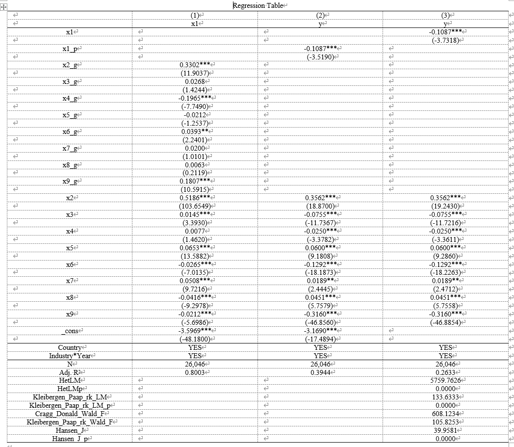
------------------------------------------------------------------------------ | Robust y | Coefficient std. err. t P>|t| [95% conf. interval] -------------+---------------------------------------------------------------- x1 | -.0958878 .0328708 -2.92 0.004 -.1603431 -.0314325 x2 | .3531729 .0213118 16.57 0.000 .3113833 .3949625 x3 | -.0767336 .007376 -10.40 0.000 -.0911971 -.0622702 x4 | -.0302413 .0083046 -3.64 0.000 -.0465255 -.0139571 x5 | .0566474 .0073346 7.72 0.000 .0422652 .0710295 x6 | -.134026 .0080818 -16.58 0.000 -.1498734 -.1181787 x7 | .0218564 .0087345 2.50 0.012 .0047292 .0389836 x8 | .042576 .0087935 4.84 0.000 .0253332 .0598188 x9 | -.3142137 .0076184 -41.24 0.000 -.3291524 -.299275 ------------------------------------------------------------------------------ Underidentification test (Kleibergen-Paap rk LM statistic): 111.379 Chi-sq(8) P-val = 0.0000 ------------------------------------------------------------------------------ Weak identification test (Cragg-Donald Wald F statistic): 455.554 (Kleibergen-Paap rk Wald F statistic): 78.984 Stock-Yogo weak ID test critical values: 5% maximal IV relative bias 20.25 10% maximal IV relative bias 11.39 20% maximal IV relative bias 6.69 30% maximal IV relative bias 4.99 10% maximal IV size 33.84 15% maximal IV size 18.54 20% maximal IV size 13.24 25% maximal IV size 10.50 Source: Stock-Yogo (2005). Reproduced by permission. NB: Critical values are for Cragg-Donald F statistic and i.i.d. errors. ------------------------------------------------------------------------------ Hansen J statistic (overidentification test of all instruments): 30.013 Chi-sq(7) P-val = 0.0001 ------------------------------------------------------------------------------ Instrumented: x1 Included instruments: x2 x3 x4 x5 x6 x7 x8 x9 Excluded instruments: x2_g x3_g x4_g x5_g x6_g x7_g x8_g x9_g Partialled-out: _cons nb: total SS, model F and R2s are after partialling-out; any small-sample adjustments include partialled-out variables in regressor count K ------------------------------------------------------------------------------
Absorbed degrees of freedom: -----------------------------------------------------+ Absorbed FE | Categories - Redundant = Num. Coefs | -------------+---------------------------------------| Country | 15 1 14 | Ind_year | 2629 2629 0 *| -----------------------------------------------------+ * = FE nested within cluster; treated as redundant for DoF computation
. est store m3
. . * First stage . reghdfe x1 x2_g-x9_g x2-x9, a(Country Ind_year) cl(Ind_year) (MWFE estimator converged in 8 iterations)
HDFE Linear regression Number of obs = 20,537 Absorbing 2 HDFE groups F( 16, 2628) = 909.28 Statistics robust to heteroskedasticity Prob > F = 0.0000 R-squared = 0.8245 Adj R-squared = 0.7984 Within R-sq. = 0.5411 Number of clusters (Ind_year) = 2,629 Root MSE = 0.4494
* Install
net install command, from("https://raw.githubusercontent.com/codefoxs/Stata-personal/main/lewbel/") replace

* Version
which lewbel
5 参考文献
Lewbel, A. (2012). Using Heteroscedasticity to Identify and Estimate Mismeasured and Endogenous Regressor Models. Journal of Business & Economic Statistics, 30(1), 67–80. https://doi.org/10.1080/07350015.2012.643126